Missing Data Imputation Using Boston Housing Dataset
- 15 minsMost of the datasets inevitably contain missing data and in most cases, those missing values are excluded from the analysis. This can limit the amount of information available, especially if the dataset contains many inputs with missing values, and could potentially bias the results. One way around the problem of missing data is imputation step that is done prior to modeling or doing any forms of analysis. In this blog post I want to take a look at a practical way of imputation and show that sometimes even simple method can take us far without affecting model’s performance. The three missing data patterns we focus here are:
-
Missing Completely at Random (MCAR) indicates that there is no relationship between the “missingness” of the data and any observed or missing values. The propensity for a data point to be missing is completely random, some data are not more likely to be missing than others.
-
Missing at Random (MAR) suggests that there is a systematic relationship between the propensity of missing values and the observed data. In other words, whether an observation is missing is not related to the missing values, but it is related to the values of an observed variable. For example, when weight information is missing for women more than men as men are more likely to reveal their weight than women.
-
Missing Not at Random (MNAR) implies that there is a relationship between the propensity of a value to be missing and its values. For example, when education field is missing for the people with the lowest education.
One important consideration in choosing imputation method is the missing data mechanism since different approaches have different assumptions about the mechanism.
In most datasets, it is likely that more than one variable will have missing data and they may not all have the same missing data mechanism. It is worthwhile to diagnose the mechanism for each variable with missing data before choosing an approach.
The imputation methods I will use here are mean, median and mode, where missing values are replaced with an average, median and mode of the non-missing data correspondingly. While there are more complex methods out there I want to focus on these three and show how model is affected when you use this simple and cheap way of inferring missing values.
Boston Housing Dataset
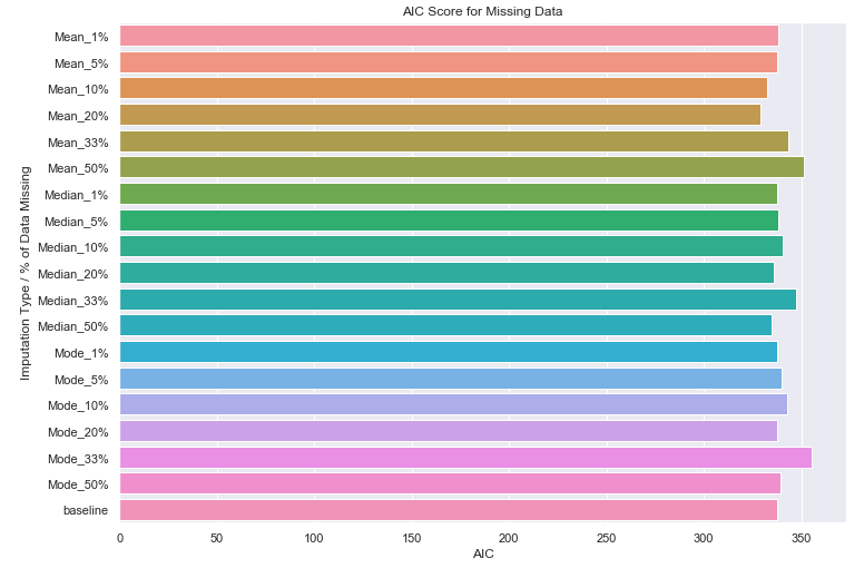
I will use The Boston Housing Dataset available in Sklearn to first fit a linear regressor and calculate the Akaike Information Criterion (AIC) metric that will serve as our baseline for comparison. We will first use the MCAR mechanism to replace the present value with a NaN for 1, 5, 10, 20, 33, and 50% of the data within a single column selected at random. For each set of missing data, we will perform an imputation of the missing value using mean, median and mode methods. We will then perform a fit with the imputed data for each case and compare the goodness of fit to the baseline.
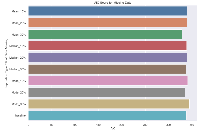
Next, we will use the MAR mechanism to create missing data. We will take two different columns at random and create three sets of missing data (10, 20, and 30% missing) while controlling for a third variable. We will then perform an imputation of the missing values for each set, fit the imputed data and compare the results to the baseline.
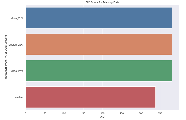
Finally, we will create a dataset in which 25% of the data is missing for a single column using the MNAR mechanism. Similarly, we will impute the missing data, fit the results and compare them to the baseline.
Let’s begin by fetching the Boston Housing data using Sklearn.
1
2
3
4
5
6
7
8
9
10
11
12
13
14
15
16
import random
import numpy as np
import pandas as pd

from sklearn.datasets import load_boston
from sklearn.linear_model import LinearRegression
from sklearn.model_selection import train_test_split
from sklearn.metrics import mean_squared_error, median_absolute_error
from sklearn.impute import SimpleImputer

import seaborn as sns

boston = load_boston()

# View the data descriptions
print(boston.DESCR)
The Boston Housing data contains 506 observations with 14 variables. The last variable, PRICE is the target variable. The original dataset does not contain any missing attribute values.
1
2
3
4
5
# Display the first 5 observations
bos = pd.DataFrame(boston.data)
bos.columns = boston.feature_names
bos['PRICE'] = boston.target
bos.head()

Baseline Model
Let’s fit a linear regression using our training data and define a function that calculates the AIC metric.
1
2
3
4
5
6
7
8
9
10
11
12
13
14
15
16
17
18
19
20
21
22
23
24
25
26
def calculate_aic(model, X, y):
    """Calculates Akaike Information Criterion
    (see https://machinelearningmastery.com/probabilistic-model-selection-measures/)"""
    mse = mean_squared_error(y, model.predict(X))
    num_params = len(model.coef_) + 1
    n = len(y)
    aic = n * np.log(mse) + 2 * num_params
    return aic

def fit_and_evaluate_lm(X, y):
    """
    Fits Linear Regression model. Calculates AIC, R2 and Median Absolute Error
    """
    # Create train and test splits from the data
    X_train, X_test, Y_train, Y_test = train_test_split(X, y, test_size = 0.2, random_state=5)
    # Perform Linear Regression
    base_model = LinearRegression()
    base_model.fit(X_train, Y_train)
    #evaluate goodness of fit and loss,
    #let's use both metrics, because median_absolute_error is less sensitive to outliers
    return {
        "AIC": calculate_aic(base_model, X_test, Y_test)
    }

base_model_results = fit_and_evaluate_lm(boston.data, boston.target)
base_model_results
{'AIC': 337.90443811267414}Based on the results above, we’ve our baseline AIC is 337.90.
MCAR
To simulate missing data we will create a function that replaces some portion of the data for a single column with a NAN.
1
2
3
4
5
6
7
def nans_at_random(X, column_idx, percentage_nan):
    """Replace values of X with a NAN completely at random"""
    X = X.copy()
    for i in range(X.shape[0]):
        if np.random.rand() < percentage_nan:
            X[i, column_idx] = np.nan
    return X
For the 1, 5 10, 20, 33, and 50% percentage values provided, we use the 3 imputation methods (mean, median, and mode) and calculate AIC.
1
2
3
4
5
6
7
8
9
10
11
12
13
14
15
16
17
percentages = [.01, .05, .1, .2, .33, .5]
imputation_methods = ['Mean', 'Median', 'Mode']

completely_at_random_results = {}
for m in imputation_methods:
    for p in percentages:
        column_index = np.random.randint(0, boston.data.shape[1] - 1)
        data = nans_at_random(boston.data, column_index, p)
        imp_mean = SimpleImputer(missing_values=np.nan, strategy='mean')
        results = fit_and_evaluate_lm(imp_mean.fit_transform(data), boston.target)
        completely_at_random_results[f'{m}_{p*100:.0f}%'] = results

completely_at_random_results['baseline'] = base_model_results

ax = sns.barplot(y=list(completely_at_random_results.keys()),
            x=list(map(lambda x: x['AIC'], completely_at_random_results.values())))
_ = ax.set(title='AIC Score for Missing Data', xlabel='AIC', ylabel='Imputation Type / % of Data Missing')

You can see that for the 18 regression models that we fit to imputed data, we do not notice any significant performance degradation when compare these model to our baseline.
MAR
To simulate MAR we create a new function that is similar to nans_at_random. In this function a value in a random column is replaced with NaN if the value in the control column is below the control column mean (i.e if Variable Z is > 30, than Variables X, Y are randomly missing). Control column and imputed columns are chosen at random.
1
2
3
4
5
6
7
8
def nans_at_random_with_control(X, column_idx, control_column, percentage_nan, ):
    """Replace values of X with a NAN completely at random when controlled for a third variable"""
    mean = np.mean(X[:, control_column])
    X = X.copy()
    for i in range(X.shape[0]):
        if np.random.rand() < percentage_nan and X[i, control_column] < mean:
            X[i, column_idx] = np.nan
    return X
Let’s runs with 10%, 20% and 30% missing data imputed, perform a fit and compare the goodness of fit to our baseline.
1
2
3
4
5
6
7
8
9
10
11
12
13
14
15
16
17
18
19
20
21
22
23
percentages = [.1, .2, .3]
imputation_methods = ['Mean', 'Median', 'Mode']

at_random_results_with_control = {}
for m in imputation_methods:
    for p in percentages:
        indexes = list(range(0, boston.data.shape[1] - 1))
        column_index1 = random.choice(indexes)
        indexes.remove(column_index1)
        column_index2 = random.choice(indexes)
        indexes.remove(column_index2)
        control_column = random.choice(indexes)
        data = nans_at_random_with_control(boston.data, column_index1, control_column, p)
        data = nans_at_random_with_control(data, column_index2, control_column, p)
        imp_mean = SimpleImputer(missing_values=np.nan, strategy='mean')
        results = fit_and_evaluate_lm(imp_mean.fit_transform(data), boston.target)
        at_random_results_with_control[f'{m}_{p*100:.0f}%'] = results

at_random_results_with_control['baseline'] = base_model_results

ax = sns.barplot(y=list(at_random_results_with_control.keys()),
            x=list(map(lambda x: x['AIC'], at_random_results_with_control.values())))
_ = ax.set(title='AIC Score for Missing Data', xlabel='AIC', ylabel='Imputation Type / % of Data Missing')

Again, we do not noticed any significant performance degradation in the goodness of fit even with 30% missing data imputed!
MNAR
Finally, we create a function that replaces the first 25% of rows with a NaN value for a given column. This function is applied to some randomly chosen column. We then calculate our goodness of fit the same way as we did before.
1
2
3
4
5
6
def nans_not_at_random(X, column_idx, percentage_nan):
    """Replace first N rows of X with a NAN"""
    pos = int(X.shape[0] * percentage_nan)
    X = X.copy()
    X[:pos] = np.nan
    return X
Let’s find the results and compare to a baseline
1
2
3
4
5
6
7
8
9
10
11
12
13
14
15
16
17
percentages = [.25]
imputation_methods = ['Mean', 'Median', 'Mode']

not_at_random_results = {}
for m in imputation_methods:
    for p in percentages:
        column_index = random.choice(list(range(0, boston.data.shape[1] - 1)))
        data = nans_not_at_random(data, column_index, p)
        imp_mean = SimpleImputer(missing_values=np.nan, strategy='mean')
        results = fit_and_evaluate_lm(imp_mean.fit_transform(data), boston.target)
        not_at_random_results[f'{m}_{p*100:.0f}%'] = results

not_at_random_results['baseline'] = base_model_results

ax = sns.barplot(y=list(not_at_random_results.keys()),
            x=list(map(lambda x: x['AIC'], not_at_random_results.values())))
_ = ax.set(title='AIC Score for Missing Data', xlabel='AIC', ylabel='Imputation Type / % of Data Missing')

This time there is a noticeable degradation in performance for all 3 imputation methods when compared to the baseline model.
Conclusion
It turned out that when we have a data set with missing values, and the data is missing at random you can expect only a slight degradation in overall performance of your statistical model when you impute your data using a very simple mechanizm. Additionally, for both the MCAR and MAR mechanisms, the percentage of data missing does not seem to have any noticeable effect on overall performance.
If you want to use more sophisticated method to infer missing values check out book Missing Data (Quantitative Applications in the Social Sciences) by Paul D. Allison, but more complex methods will likely require more development time that you will have to subtract from other important steps like data cleaning and more complex models.
Sources
- “How to Diagnose the Missing Data Mechanism”, Karen Grace-Martin.
- “Missing Data (Quantitative Applications in the Social Sciences)”, Paul D. Allison
- The Boston Housing Dataset
- Introduction to AIC — Akaike Information Criterion
