Machine Learning in Rust, Linear Regression

Any practicing data scientist is familiar with such libraries as Scikit-learn, NumPy and SciPy. But how about similar libraries in Rust, are there any good crates that can successfully be used to create machine learning applications using this blazingly fast and memory-efficient programming language? In my first blog post, dedicated to machine learning in Rust I will show how you can implement a linear regressor from scratch. I will also demonstrate some useful tools you can use to implement many other statistical learning algorithms in pure Rust.

At the end, machine learning is not hard if you have the right set of tools handy, and learning from data in Rust has its own unique benefits that are not available in other programming languages!

Part I. Machine Learning Refresher

You don’t need any prior experience in machine learning to follow my code but we need to spend some time to go over some important ideas behind statistical modeling. If you are familiar with these concepts feel free to skip this section.

First, let’s answer the question what is statistical learning? Let’s say we observe a quantitative response \(Y\) and some attributes, \(x_1, x_2, . . . , x_m\) that correspond this response. For example, let’s say you have a house that has some price and this house has 4 rooms, 2 bathrooms. Attributes of the house, like number of rooms and bathrooms are called predictors, while house price is called a target or a response. We think there might be some relationship between predictors and house price. This relationship can be written as a function, that we call a model.

\[y = f(X) + \epsilon\]

Since this function does not represent this relationship exactly there is always some irreducible error, \(\epsilon\) that we hope can be ignored in most cases.

Usually you don’t have just one sample but many. For example, instead of one house you might get a dataset with multiple houses, each with its own set of predictors and a price. When we stack our predictors vertically, one on top of another we get a matrix \(X\) with predictors, along with a column vector Y. This matrix and a column vector becomes our dataset.

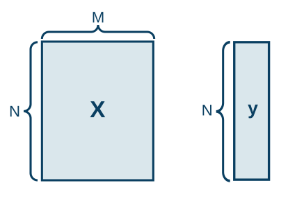
In this example we have a dataset with house attributes and prices, collected by the U.S Census Service in the area of Boston, MA. This dataset has 13 numerical and categorical attributes. We want to predict a house price from these attributes.

We use statistical models to solve problems and there are multiple ways to categorize these problems. For example, when your target \(Y\) is quantitative (in other words numerical), you can build a regression model that predicts this value from \(X\). When \(Y\) is categorical, your only option is a classifier that can predict a class \(Y\) from \(X\).

Model testing is an integral part of statistical modeling process because all models are not ideal and you should understand how far your predictions are from true values to set proper expectations and manage risks correctly. One common technique to estimate irreducible error is to split your data into training and test datasets. You use training dataset to fit your model and you use test dataset to estimate error by comparing predicted values to true values.

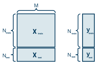
So how do you choose a model that captures relationship between X and Y? What are the parameters of this model? How do we estimate these parameters?

These are the key questions that you ask yourself when you develop a statistical model. When you solve a machine learning problem first thing you try to understand is what category this problem falls into: can you do supervised learning? Is it a classifier or regressor that your client needs? What kind of existing algorithm fits my data better?

The answer to all these question will depend on your problem and your data, but what you will need are libraries with wide variety of algorithms that you can use to model relationship between \(Y\) and \(X\). Languages like Python and R provide a vast ecosystem of tools that can be used by engineers to design and implement statistical models. Most of these tools use methods developed in 4 branches of mathematics that you can see on the figure below. The good news is that in Rust you’ll find mature libraries that provide methods in at least 2 of these critical branches: optimization and linear algebra.

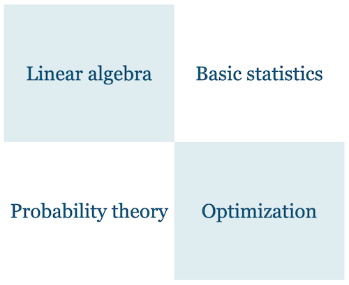
In this and next blog posts I will focus on one specific approach to supervised learning, linear models, that assumes there is approximately a linear relationship between \(X\) and \(Y\). I will use this simple modeling technique to demonstrate Rust crates that you can use to implement other machine learning algorithms as well. Besides, linear models are popular in machine learning and have many useful properties like great interpretability, fast implementation and great generalization power.

In linear model, when we have just one predictor \(x_1\), we model relationship between \(X\) and \(Y\) as a line that intercepts axis Y at some point beta 0 and has a slope beta 1.

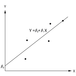
When we have 2 predictors, our line becomes a plane that is defined by 2 parameters, \(\beta_1\) and \(\beta_2\) and intercepts axes Y at point \(\beta_0\). When you fit a linear model to your data your goal is to find values for model parameters, \(\beta\).

\[ \begin{equation} \boldsymbol{y} = \boldsymbol{X}\beta + \epsilon \end{equation} \]

Part II. Linear Regression in Rust

Let’s see how we would fit a linear model in Python. To demonstrate regression I will use The Boston Housing Dataset and I want to predict a house price from house attributes.

1
2
3
4
import numpy as np
from sklearn.datasets import load_boston

boston = load_boston()

Our first step would be to separate predictors, \(X\) from target \(Y\) and to split our dataset into test and training sets.

1
2
3
4
5
6
7
8
9
10
11
12
import pandas as pd
from sklearn.model_selection import train_test_split

bos = pd.DataFrame(boston.data)
bos.columns = boston.feature_names
bos['PRICE'] = boston.target

X = bos.drop('PRICE', axis=1).values
y = bos.PRICE.values

X_train, X_test, y_train, y_test = train_test_split(X, y, test_size = 0.2)   
X_train.shape, X_test.shape, y_train.shape, y_test.shape

Now we are ready to fit linear regressor to the training portion of \(X\) and \(Y\). Linear regressor is defined in Scikit Learn package. This package provides big selection of traditional machine learning algorithms and is a go-to library for machine learning that is widely used in the industry. With Scikit Learn we can fit linear regressor to our data in one line.

1
2
from sklearn.linear_model import LinearRegression
lr = LinearRegression().fit(X_train, y_train)

To evaluate performance of our regressor we will use mean absolute error that calculates mean absolute difference between predicted and true values.

\[mse(y, \hat{y}) = \frac{1}{n_{samples}} \sum_{i=1}^{n_{samples}} \lvert y_i - \hat{y_i} \rvert\]

We calculate mean absolute error using test dataset and get 3.4

1
2
from sklearn.metrics import mean_absolute_error
print(mean_absolute_error(y_test, lr.predict(X_test)))

3.447122276148069

We can also print parameters of our model.

1
print("coef: {}, intercept: {}".format(lr.coef_, lr.intercept_))

coef: [-1.09345106e-01  5.14771860e-02 -1.35771811e-02  3.11370157e+00
 -1.53107579e+01  3.54796861e+00 -4.78707187e-03 -1.49453646e+00
  3.17255788e-01 -1.20148597e-02 -9.28169726e-01  1.03065117e-02
 -5.58857305e-01], intercept: 37.03977851074369

The code I’ve demonstrated uses several Python packages, but the most notable package by far is NumPy. NumPy is a backbone of most libraries for machine learning and scientific computing in Python because NumPy provides a toolset for manipulating n dimensional arrays as well as linear algebra routines. Scikit Learn relies heavily on NumPy to compute parameters of the model when you call fit and predict methods.

We would need a similar library if I want to train and run our statistical models in Rust. Luckily, there are at least 2 great crates in Rust that we can use to manipulate n dimensional arrays: nalgebra and ndarray. While these libraries provide slightly different functionality we could use both interchangeably for our purpose. One important difference between these two libraries is that nalgebra supports only 2D and 1D arrays while ndarray support arrays of arbitrary size. The other difference is that you do not need BLAS and LAPACK backend to solve linear equations and decompose matrices when you use nalgebra.

We start by importing nalgebra structs and traits where data manipulation functions are defined.

1
use nalgebra::{DMatrix, DVector, Scalar};

We read the file with Boston Housing dataset. Unfortunately, nalgebra does not provide a function to read data from CSV file but it is not hard to implement one yourself.

1
2
3
4
5
6
7
8
9
10
11
12
13
14
15
16
17
18
19
20
21
22
23
24
25
26
27
28
29
30
31
32
33
34
35
36
37
38
39
40
use std::io::prelude::*;
use std::io::BufReader;
use std::fs::File;
use std::str::FromStr;

fn parse_csv<N, R>(input: R) -> Result<DMatrix<N>, Box<dyn std::error::Error>>
  where N: FromStr + Scalar,
        N::Err: std::error::Error,
        R: BufRead
{
  // initialize an empty vector to fill with numbers
  let mut data = Vec::new();

  // initialize the number of rows to zero; we'll increment this
  // every time we encounter a newline in the input
  let mut rows = 0;

  // for each line in the input,
  for line in input.lines() {
    // increment the number of rows
    rows += 1;
    // iterate over the items in the row, separated by commas
    for datum in line?.split_terminator(",") {
      // trim the whitespace from the item, parse it, and push it to
      // the data array
      data.push(N::from_str(datum.trim())?);
    }
  }

  // The number of items divided by the number of rows equals the
  // number of columns.
  let cols = data.len() / rows;

  // Construct a `DMatrix` from the data in the vector.
  Ok(DMatrix::from_row_slice(rows, cols, &data[..]))
}

let file = File::open("../data/creditcard.csv").unwrap();
let bos: DMatrix<f64> = parse_csv(BufReader::new(file)).unwrap(); 
println!("{}", bos.rows(0, 5));

This is how our data looks like once it is represented as a 2 dimensional matrix. The leftmost column is a house price while the rest of the columns are the attributes of a house.

We separate predictors from price using matrix manipulation methods defined in nalgebra.

1
2
let x = bos.columns(0, 13).into_owned();
let y = bos.column(13).into_owned();

To split data into training/test sets we need to use a function defined in another Rust crate, Smartcore.

1
2
use smartcore::model_selection::train_test_split;
let (x_train, x_test, y_train, y_test) = train_test_split(&x, &y.transpose(), 0.2);

So how can we fit linear regression in Rust? From linear algebra we know that one way to solve system of linear equations

\[Ax = b\]

is by taking an inverse of \(A\)

\[x = A^{-1}b\]

If you compare the formula that represents linear regression to this expression you will see that all we need to do to find parameters of linear regression is to take an inverse of X

\[X\beta = y\] \[\beta = X^{-1}y\]

One problem with solving this equation directly is that for a tall and skinny matrices, where you have more rows than columns, there will likely be no exact solutions. So one of the tricks that we can use to find an approximate solution is to convert X into a square matrix by multiplying our equation by \(X^T\) transpose from both sides. Now the solution can be found by taking an inverse of \(X^TX\)

\[X^TX\beta = X^Ty\] \[\beta = (X^TX)^{-1}X^Ty\]

Let’s see whether we’ll arrive to the same parameter values if we apply this formula in Rust. Let’s define A and b

1
2
let a = x_train.clone().insert_column(13, 1.0).into_owned();
let b = y_train.clone().transpose();

When we apply the formula from the previous slide to our data we get similar coefficients and intercept!

1
2
3
4
let x = (a.transpose() * &a).try_inverse().unwrap() * &a.transpose() * &b;
let coeff = x.rows(0, 13);
let intercept = x[(13, 0)];
println!("coeff: {}, intercept: {}", coeff, intercept);

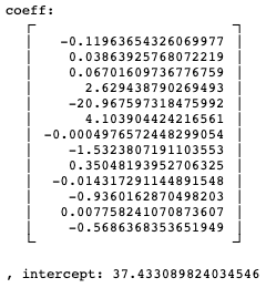
Notice that coefficients and intercept are very close to the values we’ve got in Python. The reason why numbers are not the same is because our train/test split in Rust is different from train/test split in Python due to randomization.

One problem with this approach for estimating model parameters is the matrix inverse that is both computationally expensive and numerically unstable. An alternative approach is to use a matrix decomposition to avoid this operation. The matrix decomposition breaks a matrix down into its constituent elements. There are many decomposition methods out these but for this example I will use QR decomposition that can break our matrix A into matrices Q and R.

\[X = QR\]

Stepping over all of the derivation, the coefficients can be found using the Q and R matrices using this formula.

\[\beta = R^{-1}Q^Ty\]

This approach still involves a matrix inversion, but in this case only on the simpler matrix R.

In Rust both ndarray and nalgebra provide multiple matrix decomposition methods as well. This is how we would decompose matrix and solve the equation in Rust using nalgebra.

1
2
3
4
5
6
let qr = a.qr();
let (q, r) = (qr.q().transpose(), qr.r());        
let x = r.try_inverse().unwrap() * &q * &b;
let coeff = x.rows(0, 13);
let intercept = x[(13, 0)];
println!("coeff: {}, intercept: {}", coeff, intercept);

We’ve got the same values for coefficients and intercept again! Now that we have parameters of linear regressor how do we estimate house prices? We just multiply our parameter estimates, \(\hat{\beta}\) by \(X\)!

\[\hat{y} = X\hat{\beta}\]

1
2
let y_hat = (x_test * &coeff).add_scalar(intercept);
println!("mae: {}", mean_absolute_error(&y_test, &y_hat.transpose()));

mae: 3.1081864959381837

Mean absolute error is very close to the error we’ve calculated in Python. Again, the reason why haven’t got the same number is because our train/test split in Rust is not the same as in Python.

Conclusion

The fact that we were able to fit a linear regressor to Boston Housing dataset in Rust is remarkable. What makes our result even better is that our algorithm achieved the same performance as the Scikit Learn’s implementation and that we had to write very little code to estimate parameters of our model. Most of the work is done by one of the linear algebra crates that is provided by Rust ecosystem. The good news is that many other core machine learning algorithms rely on linear algebra routines for parameter estimation. You will use the same set of tools if you want to implement algorithms like PCA, SVD and Ridge Regression in Rust.

In my next post dedicated to machine learning in Rust I will show you some additional tools that are crutial if you want to fit statistical models to your data. Stay tuned!

Sources

• “An Introduction to Statistical Learning”, James G., Witten D., Hastie T., Tibshirani R.
• The Boston Housing Dataset
• nalgebra: linear algebra library for Rust.
• ndarray: an N-dimensional array with array views, multidimensional slicing, and efficient operations
• SmartCore: a comprehensive library for machine learning and numerical computing in Rust
• Source code

Vlad Orlov

Data Scientist, Open Source Contributor, Technology Enthusiast

Tweet Share